Applying the Composite Trapezoidal Rule to Fredholm Integral Equations of the Second Kind

July 1, 2019

Fredholm integral equations of the second kind are of the form:

$$u(x) = f(x) + \int_{a}^{b} K(x,t)u(t)dt$$

Given $f(x)$ and $K(x,t)$, can we find the solution for the unknown function $u(x)$? The most difficult part of this problem is evaluating the integral $\int_{a}^{b} K(x,t)u(t) dt$, which often has no analytical solution if the kernel function $K(x,t)$ is complicated. It is helpful to approach these problems numerically.

One naive approach to this problem is to try to approximate $\int_{a}^{b} K(x,t)u(t) dt$. We will solve it using the composite trapezoidal rule. Assuming a uniform grid with $n$ equal partitions and step-size $h=\frac{b-a}{n}$, the composite trapezoidal rule is as stated:

$$\int_{a}^{b} f(x)dx \approx \frac{h}{2}\left(f(x_0) + 2\sum_{i=1}^{n-1}f(x_i) + f(x_n)\right)$$

where $x_i \in [a,b]$ for $i = 0, 1, \dots, n$. When we apply the composite trapezoidal rule to our integral, we get

$$\int_{a}^{b}K(x, t)u(t)dt = \frac{h}{2}\left(K(x, x_0)u(x_0) + 2\sum_{i=1}^{n-1}K(x, x_i)u(x_i) + K(x, x_n)u(x_n)\right)$$

By substituting this information into our original equation, we can define $u(x)$ in the following way:

$$u(x) = f(x) + \frac{h}{2}\left(K(x, x_0)u(x_0) + 2\sum_{i=1}^{n-1}K(x, x_i)u(x_i) + K(x, x_n)u(x_n)\right)$$

When we evaluate $u(x)$ at all the evenly spaced nodes $x_0, x_1, \dots , x_n \in [a,b]$, we can construct the system of equations:

$$\begin{aligned} u(x_0) &= f(x_0) + \frac{h}{2}\left(K(x_0, x_0)u(x_0) + 2\sum_{i=1}^{n-1}K(x_0, x_i)u(x_i) + K(x_0, x_n)u(x_n)\right) \\ u(x_1) &= f(x_1) + \frac{h}{2}\left(K(x_1, x_0)u(x_0) + 2\sum_{i=1}^{n-1}K(x_1, x_i)u(x_i) + K(x_1, x_n)u(x_n)\right) \\ &\vdots \\ u(x_{n-1}) &= f(x_{n-1}) + \frac{h}{2}\left(K(x_{n-1}, x_0)u(x_0) + 2\sum_{i=1}^{n-1}K(x_{n-1}, x_i)u(x_i) + K(x_{n-1}, x_n)u(x_n)\right) \\ u(x_n) &= f(x_n) + \frac{h}{2}\left(K(x_n, x_0)u(x_0) + 2\sum_{i=1}^{n-1}K(x_n, x_i)u(x_i) + K(x_n, x_n)u(x_n)\right) \\ \end{aligned}$$

Solving this system yields the values for $u(x_0), u(x_1),\dots,u(x_n)$. The matrix form of this system looks like

$$\left(I_{n+1} - \frac{h}{2}\begin{bmatrix} K(x_0, x_0) & 2K(x_0, x_1) & \cdots & 2K(x_0, x_{n-1}) & K(x_0, x_n) \\ K(x_1, x_0) & 2K(x_1, x_1) & \cdots & 2K(x_1, x_{n-1}) & K(x_1, x_n) \\ \vdots & \vdots & \ddots & \vdots & \vdots \\ K(x_{n-1}, x_0) & 2K(x_{n-1}, x_1) & \cdots & 2K(x_{n-1}, x_{n-1}) & K(x_{n-1}, x_n) \\ K(x_n, x_0) & 2K(x_n, x_1) & \cdots & 2K(x_n, x_{n-1}) & K(x_n, x_n) \end{bmatrix}\right) \begin{bmatrix} u(x_0) \\ u(x_1) \\ \vdots \\ u(x_{n-1}) \\ u(x_n) \end{bmatrix} = \begin{bmatrix} f(x_0) \\ f(x_1) \\ \vdots \\ f(x_{n-1}) \\ f(x_n) \end{bmatrix}$$

where $I_{n+1}$ is the identity matrix of size $n+1$.

Let’s try this on an example problem. Let $u(x) = e^x-1+\int_{0}^{1}tu(t)dt$ where $f(x) = e^x-1$ and $K(x,t)=t$. The exact solution to this equation is $u(x)=e^x$¹. Let’s use $n=4$ intervals with a step-size of $h=\frac{1}{4}$. Our set of nodes will then be ${ 0, \frac{1}{4}, \frac{1}{2}, \frac{3}{4}, 1 }$. The matrix equation is

$$\begin{pmatrix}I_5 - \frac{1}{8}\begin{bmatrix} 0 & 0.5 & 1 & 1.5 & 1\\ 0 & 0.5 & 1 & 1.5 & 1\\ 0 & 0.5 & 1 & 1.5 & 1\\ 0 & 0.5 & 1 & 1.5 & 1\\ 0 & 0.5 & 1 & 1.5 & 1 \end{bmatrix} \end{pmatrix} \begin{bmatrix}u(0)\\ u(0.25)\\ u(0.5)\\ u(0.75)\\ u(1)\end{bmatrix} = \begin{bmatrix}0\\ e^{0.25}-1\\ e^{0.5}-1\\ e^{0.75}-1\\ e-1\end{bmatrix}$$

MATLAB spits out

u(0)	1.0461
u(0.25)	1.3302
u(0.5)	1.6949
u(0.75)	2.1631
u(1)	2.7644

Let’s look at a plot of our approximation versus the exact solution:

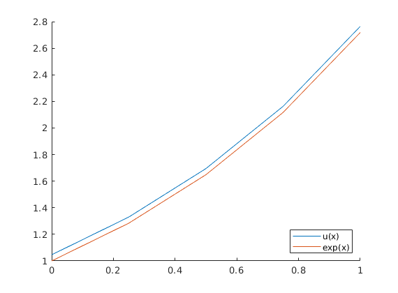
It looks okay. We can see that there is some error when we only use $4$ intervals. Let’s see if we can do better when $n=8$:

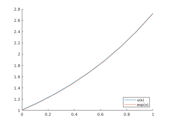
The error is much smaller, which should make sense because the composite trapezoidal rule has error of order $O(h^3)$. So when we double our steps-size, our error is $\frac{1}{8}$ed.

---